How good is each SuperBowl Square

February 11th, 2024 by Rohan Rao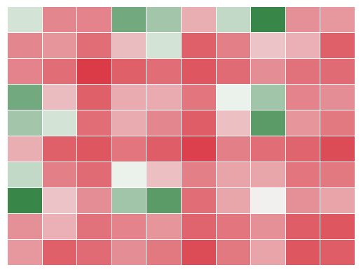

Superbowl Squares

I don’t watch much football and so most betting games around the superbowl aren’t for me but there’s one that seems fun to me and I’d naively guess doesn’t take too much football knowledge to get into called superbowl squares.

There are two main formats of this game that all generally deal with bets on the last digit of each team’s scores

At a high level you have a 10 x 10 grid of squares that that different players own, for example

png

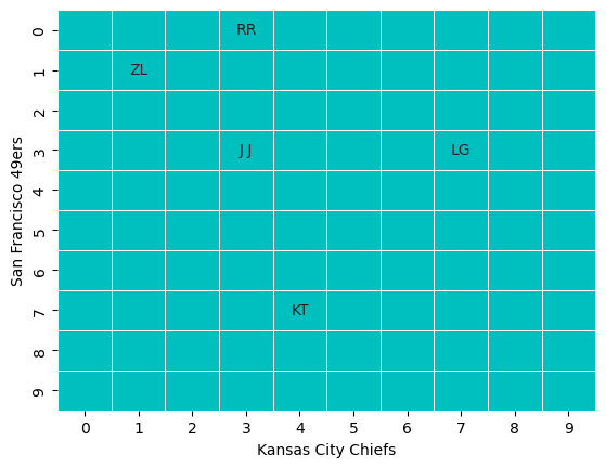
Here for example player RR owns the square with \(y\) coordinate \(0\) and \(x\) coordinate \(3\) and so (depending on the game format) they would win if the last digit of the 49er’s score was \(0\) and the last digit of the Chiefs’ score was \(3\)

To be formal about things, we start with some teams \(\mathcal{T}\) in the NFL.

We have some sort of game outcome

\(G = (A, B, Q1_A, Q2_A, Q3_A, F_A, Q1_B, Q2_B, Q3_B, F_B)\) Where \(A,B \in \mathcal{T}\) and \(Q1_A\) represents team A’s Q1 score mod 10 and so on (\(F\) indicates final score mod 10).

Quarter Format:

In this format, a square pays out in the following way

\[S^{Q}_{A,B}(x,y) = 25 \cdot \mathbb{1}_{Q1_A = x \land Q1_B = y} + 25 \cdot \mathbb{1}_{Q2_A = x \land Q2_B = y} + 25 \cdot \mathbb{1}_{Q3_A = x \land Q3_B = y} + 25 \cdot \mathbb{1}_{F_A = x \land F_B = y}\]

So pretty much for each quarter score that your square matches you get 25 bucks.

Full Game Format:

In this format

\[S^{G}_{A,B}(x,y) = 100 \cdot \mathbb{1}_{F_A = x \land F_B = y}\]

So you get 100 bucks at the end of the game if you had the winning square

Problem Setting:

Given a dataset of historical NFL box scores the goal here is to estimate what squares are worth (in expectation)

Elements from the dataset look something like:

Team	Q1 % 10	Q2 % 10	Q3 % 10	F % 10
Atlanta Falcons	3	2	2	7
Green Bay Packers	3	2	9	9

We could treat this game outcome as

\((Falcons, Packers, 3, 2, 2, 7, 3, 2, 9, 9)\) or \((Packers, Falcons, 3, 2, 9, 9, 3, 2, 2, 7)\) or randomly pick one of these. It seems reasonable to pick an ordering based on information available before seeing game scores. A few reasonable options:

Randomize Team Ordering (enforcing some symmetry)
Keep ordering Consistent with NFL Data

Option (2) has benefits if the NFL website picks an ordering based on info we would know before we pick squares (like home / away games). That being said I’m not sure how the ordering of the dataset is and so it seems safer and easier to reason about to go with (1).

We thus ignore home vs away games / ordering effects so given two teams \(a, b \in \mathcal{T}\) then \((a, b, x_1, x_2, x_3, x_4, x_5, x_6, x_7, x_8)\) has the same probability as \((b, a, x_5, x_6, x_7, x_8, x_1, x_2, x_3, x_4)\) (conditioned on \(a\) and \(b\) respectively) and \(S_{a,b}(x,y)\) and \(S_{b,a}(y,x)\) have the same distribution. Furthermore assuming we have some probability distribution over game outcomes as defined above the marginal probability of seeing teams \((a,b)\) is the same as \((b,a)\).

Here’s some examples of the data

NFL Data from https://thedatajocks.com/data/

                 Team  Q1  Q2  Q3  Final
0      Houston Texans   7   0   0     20
1  Kansas City Chiefs   0  17   7     34
2    Seattle Seahawks  14   0  14     38
3     Atlanta Falcons   3   9   0     25
4   Green Bay Packers   3  19   7     43

Processed to get ones digit:  
                 Team  Q1  Q2  Q3  Final
0      Houston Texans   7   7   7      0
1  Kansas City Chiefs   0   7   4      4
2    Seattle Seahawks   4   4   8      8
3     Atlanta Falcons   3   2   2      5
4   Green Bay Packers   3   2   9      3


Example of Game: 
                 Team  Q1  Q2  Q3  Final
0      Houston Texans   7   7   7      0
1  Kansas City Chiefs   0   7   4      4



Processed Into Row Observation:
[7, 7, 7, 0, 0, 7, 4, 4]

One more issue with modeling the game outcomes as some probability distribution as defined above is that the (A, B) pairs are not random but chosen by the NFL schedule.

The NFL uses a strict scheduling algorithm to determine which teams play each other from year to year, based on the current division alignments and the final division standings from the previous season. (Wikipedia)

And since we just have the whole season results, the \((A,B)\) pairs aren’t independently drawn in our dataset. If we assume though that \((Q1_A, Q2_A, Q3_A, F_A, Q1_B, Q2_B, Q3_B, F_B)\) is independent of A and B (maybe a strong assumption) and we furthermore assume that each game’s scores were independent from each other and drawn from the same distribution, then we can think of our dataset as being IID draws of

\[X = (Q1_A, Q2_A, Q3_A, F_A, Q1_B, Q2_B, Q3_B, F_B)\]

To summarize the assumptions made above are

Game scores are independent between games
Game scores are symmetric with respect to permuting the team ordering (the ordering doesn’t give you info)
Game scores are identically distributed (i.e. teams playing don’t change the distribution)

My general sense is that (1) might be reasonable, (2) is true by construction (3) idrk (I’m not a big football guy)

Either way now we can rewrite \(S_{A,B}(x,y)\) as \(S(x,y)\) and we note that \(\mathbb{E}[S(x,y)] = \mathbb{E}[S(y,x)] = \mu\). In fact the distributions of \(S(x,y)\) and \(S(y,x)\) are identical in our model due to assumption (2).

Finally we want to estimate \(\mu\), lets call this estimate \(\hat{\mu}\)

Estimating The Mean

From each observed \(\hat{X}_i\) we can compute \(\hat{S}_i(x,y)\) or the empirical payoff of that square. From this its an unbiased estimate to compute \(\hat{u} = \frac{1}{n}\sum_{i = 1}^n \hat{S}_i(x,y)\) \(E[\hat{u}] = \mu\) \(Var(\hat{u}) = \frac{1}{n^2}\sum Var(S_i(x,y))\)

But since we also know that \(\mathbb{E}(S_i(x,y)) = \mathbb{E}(S_i(y,x))\) we could estimate

\[\hat{u} = \frac{1}{2n}\sum_{i = 1}^n \hat{S}_i(x,y) + \frac{1}{2n}\sum_{i = 1}^n \hat{S}_i(y,x)\]

This still has the property that \(E[\hat{u}] = \mu\)

But

\[Var(\hat{u}) = \frac{1}{4n^2}\sum Var(S_i(x,y)) + \frac{1}{4n^2}\sum Var(S_i(y,x)) + 2Cov(\frac{1}{2n}\sum_iS_i(x,y),\frac{1}{2n}\sum_iS_i(y,x))\]

And \(Cov(S_i(x,y),S_i(y,x)) < 0\) so this is actually a lower variance estimate (if \(x \neq y\) otherwise its the same)

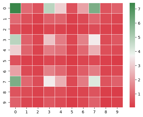
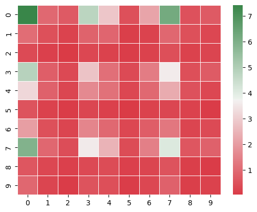
Estimated Expected Quarterly Payoff (Estimator using Symmetry)
[[7.43 1.01 0.52 4.8  3.03 0.51 2.1  6.06 0.55 0.82]
 [1.01 0.47 0.19 0.81 0.87 0.17 0.35 0.94 0.39 0.27]
 [0.52 0.19 0.03 0.32 0.23 0.08 0.23 0.43 0.18 0.16]
 [4.8  0.81 0.32 2.8  1.38 0.31 1.46 3.59 0.38 0.62]
 [3.03 0.87 0.23 1.38 1.16 0.24 0.98 2.39 0.45 0.37]
 [0.51 0.17 0.08 0.31 0.24 0.03 0.24 0.33 0.17 0.09]
 [2.1  0.35 0.23 1.46 0.98 0.24 0.73 1.34 0.25 0.34]
 [6.06 0.94 0.43 3.59 2.39 0.33 1.34 4.11 0.56 0.81]
 [0.55 0.39 0.18 0.38 0.45 0.17 0.25 0.56 0.14 0.11]
 [0.82 0.27 0.16 0.62 0.37 0.09 0.34 0.81 0.11 0.19]]

png

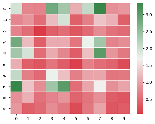
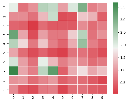
Estimated Expected Full Game Payoff (Estimator using Symmetry)
[[1.94 0.75 0.72 2.81 2.37 1.09 2.09 3.34 0.84 0.91]
 [0.75 0.87 0.53 1.22 1.94 0.41 0.69 1.28 1.12 0.41]
 [0.72 0.53 0.06 0.41 0.53 0.31 0.5  0.81 0.56 0.5 ]
 [2.81 1.22 0.41 1.06 1.06 0.59 1.72 2.4  0.72 0.81]
 [2.37 1.94 0.53 1.06 0.75 0.37 1.25 3.03 0.87 0.62]
 [1.09 0.41 0.31 0.59 0.37 0.12 0.69 0.53 0.44 0.22]
 [2.09 0.69 0.5  1.72 1.25 0.69 1.   1.03 0.59 0.62]
 [3.34 1.28 0.81 2.4  3.03 0.53 1.03 1.69 0.84 1.  ]
 [0.84 1.12 0.56 0.72 0.87 0.44 0.59 0.84 0.37 0.31]
 [0.91 0.41 0.5  0.81 0.62 0.22 0.62 1.   0.31 0.37]]

png

Estimated Expected Quarterly Payoff (Estimator Naive)
[[7.43 0.97 0.69 4.75 2.86 0.47 2.15 6.2  0.52 0.69]
 [1.05 0.47 0.22 0.84 0.92 0.14 0.22 0.95 0.47 0.31]
 [0.36 0.16 0.03 0.31 0.19 0.09 0.2  0.44 0.2  0.25]
 [4.86 0.78 0.33 2.8  1.12 0.36 1.37 3.61 0.44 0.7 ]
 [3.2  0.83 0.27 1.64 1.16 0.31 0.98 2.3  0.5  0.31]
 [0.55 0.2  0.06 0.27 0.17 0.03 0.19 0.27 0.19 0.06]
 [2.05 0.48 0.25 1.55 0.97 0.3  0.73 1.25 0.25 0.36]
 [5.92 0.94 0.42 3.58 2.48 0.39 1.44 4.11 0.59 0.81]
 [0.59 0.31 0.16 0.33 0.41 0.16 0.25 0.53 0.14 0.08]
 [0.95 0.23 0.08 0.55 0.44 0.11 0.31 0.81 0.14 0.19]]

png

Estimated Expected Full Game Payoff (Estimator Naive)
[[1.94 0.62 0.94 2.44 2.31 1.06 2.06 3.   0.75 0.94]
 [0.87 0.87 0.62 1.31 2.25 0.25 0.31 1.44 1.25 0.44]
 [0.5  0.44 0.06 0.56 0.37 0.37 0.37 0.87 0.56 0.75]
 [3.19 1.12 0.25 1.06 0.69 0.69 1.5  2.44 0.62 0.94]
 [2.44 1.62 0.69 1.44 0.75 0.5  1.19 2.75 0.75 0.5 ]
 [1.12 0.56 0.25 0.5  0.25 0.12 0.62 0.62 0.44 0.25]
 [2.12 1.06 0.62 1.94 1.31 0.75 1.   0.87 0.56 0.69]
 [3.69 1.12 0.75 2.37 3.31 0.44 1.19 1.69 1.12 1.37]
 [0.94 1.   0.56 0.81 1.   0.44 0.62 0.56 0.37 0.19]
 [0.87 0.37 0.25 0.69 0.75 0.19 0.56 0.62 0.44 0.37]]

png

might as well attempt some confidence intervals too - just to get a little color beyond a point estimate here

Confidence Intervals

We have two estimators.

\(\hat{\mu_1} = \frac{1}{n}\sum_{i = 1}^n \hat{S}_i(x,y)\) \(\hat{\mu_2} = \frac{1}{n}\sum_{i = 1}^n (\frac{1}{2}\hat{S}_i(x,y) + \frac{1}{2}\hat{S}_i(y,x))\)

Our normalized estimators can be modeled as being \(t\)-distributed \(\frac{(\hat{\mu_1} - \mu)}{s_1/\sqrt{n}} \sim t_{n-1}\) \(\frac{(\hat{\mu_2} - \mu)}{s_2/\sqrt{n}} \sim t_{n-1}\)

so we can construct estimate-level confidence intervals in the standard way and we can see that the CI’s constructed in this way are tighter for the mean of \(\hat{u_2}\). This is somewhat expected since we think that \(\hat{\mu_2}\) has lower variance

Alternatively we could bootstrap a confidence interval (though its a bit more work)

t-95%  CI Width (Quarterly Estimator using Symmetry)
Width
[[1.37 0.37 0.27 0.8  0.62 0.26 0.53 0.86 0.29 0.33]
 [0.37 0.34 0.15 0.33 0.34 0.16 0.21 0.36 0.22 0.18]
 [0.27 0.15 0.09 0.21 0.17 0.1  0.18 0.23 0.15 0.15]
 [0.8  0.33 0.21 0.88 0.42 0.2  0.47 0.68 0.23 0.29]
 [0.62 0.34 0.17 0.42 0.56 0.18 0.37 0.58 0.24 0.22]
 [0.26 0.16 0.1  0.2  0.18 0.09 0.18 0.21 0.15 0.1 ]
 [0.53 0.21 0.18 0.47 0.37 0.18 0.47 0.41 0.17 0.22]
 [0.86 0.36 0.23 0.68 0.58 0.21 0.41 1.08 0.27 0.32]
 [0.29 0.22 0.15 0.23 0.24 0.15 0.17 0.27 0.2  0.11]
 [0.33 0.18 0.15 0.29 0.22 0.1  0.22 0.32 0.11 0.23]]

t-95%  CI Width (Quarterly Estimator Naive)
Width
[[1.37 0.52 0.44 1.13 0.9  0.35 0.78 1.24 0.39 0.44]
 [0.56 0.34 0.23 0.47 0.51 0.2  0.23 0.54 0.35 0.29]
 [0.32 0.19 0.09 0.27 0.21 0.15 0.25 0.34 0.22 0.26]
 [1.13 0.48 0.33 0.88 0.54 0.3  0.62 1.02 0.35 0.44]
 [0.93 0.46 0.27 0.66 0.56 0.31 0.54 0.8  0.36 0.27]
 [0.38 0.22 0.12 0.25 0.2  0.09 0.23 0.27 0.21 0.12]
 [0.76 0.35 0.26 0.68 0.53 0.28 0.47 0.57 0.24 0.3 ]
 [1.24 0.49 0.32 0.98 0.83 0.34 0.61 1.08 0.39 0.45]
 [0.45 0.27 0.19 0.3  0.32 0.21 0.24 0.37 0.2  0.14]
 [0.51 0.24 0.14 0.39 0.34 0.16 0.29 0.47 0.18 0.23]]

Naive Width - Symmetry Width
[[ 0.    0.15  0.17  0.33  0.28  0.1   0.25  0.39  0.1   0.11]
 [ 0.18  0.    0.08  0.14  0.16  0.05  0.02  0.17  0.13  0.1 ]
 [ 0.05  0.04  0.    0.06  0.04  0.05  0.07  0.11  0.07  0.11]
 [ 0.33  0.15  0.12  0.    0.13  0.11  0.15  0.34  0.12  0.15]
 [ 0.31  0.12  0.1   0.24  0.    0.13  0.16  0.22  0.12  0.05]
 [ 0.12  0.06  0.03  0.06  0.02  0.    0.05  0.05  0.06  0.02]
 [ 0.23  0.14  0.08  0.21  0.16  0.1   0.    0.17  0.07  0.09]
 [ 0.38  0.13  0.08  0.31  0.25  0.12  0.2   0.    0.12  0.13]
 [ 0.15  0.05  0.05  0.07  0.08  0.06  0.07  0.11  0.    0.02]
 [ 0.18  0.05 -0.01  0.1   0.13  0.06  0.07  0.15  0.07  0.  ]]



t-95%  CI Width (Full Game Estimator using Symmetry)
Width
[[1.35 0.6  0.58 1.13 1.04 0.72 0.98 1.22 0.63 0.65]
 [0.6  0.91 0.5  0.76 0.95 0.44 0.57 0.77 0.73 0.44]
 [0.58 0.5  0.25 0.44 0.5  0.39 0.49 0.62 0.52 0.49]
 [1.13 0.76 0.44 1.01 0.71 0.53 0.89 1.05 0.58 0.62]
 [1.04 0.95 0.5  0.71 0.85 0.42 0.77 1.17 0.64 0.54]
 [0.72 0.44 0.39 0.53 0.42 0.35 0.57 0.5  0.46 0.32]
 [0.98 0.57 0.49 0.89 0.77 0.57 0.98 0.7  0.53 0.54]
 [1.22 0.77 0.62 1.05 1.17 0.5  0.7  1.26 0.63 0.69]
 [0.63 0.73 0.52 0.58 0.64 0.46 0.53 0.63 0.6  0.39]
 [0.65 0.44 0.49 0.62 0.54 0.32 0.54 0.69 0.39 0.6 ]]

t-95%  CI Width (Full Game Estimator Naive)
Width
[[1.35 0.77 0.94 1.51 1.47 1.01 1.39 1.67 0.85 0.94]
 [0.91 0.91 0.77 1.12 1.45 0.49 0.55 1.17 1.09 0.65]
 [0.69 0.65 0.25 0.73 0.6  0.6  0.6  0.91 0.73 0.85]
 [1.72 1.03 0.49 1.01 0.81 0.81 1.19 1.51 0.77 0.94]
 [1.51 1.24 0.81 1.17 0.85 0.69 1.06 1.6  0.85 0.69]
 [1.03 0.73 0.49 0.69 0.49 0.35 0.77 0.77 0.65 0.49]
 [1.41 1.01 0.77 1.35 1.12 0.85 0.98 0.91 0.73 0.81]
 [1.85 1.03 0.85 1.49 1.75 0.65 1.06 1.26 1.03 1.14]
 [0.94 0.98 0.73 0.88 0.98 0.65 0.77 0.73 0.6  0.42]
 [0.91 0.6  0.49 0.81 0.85 0.42 0.73 0.77 0.65 0.6 ]]

Naive Width - Symmetry Width
[[ 0.    0.18  0.36  0.38  0.43  0.29  0.41  0.45  0.21  0.29]
 [ 0.32  0.    0.27  0.36  0.51  0.05 -0.02  0.39  0.36  0.21]
 [ 0.11  0.14  0.    0.29  0.1   0.21  0.11  0.29  0.22  0.36]
 [ 0.59  0.28  0.05  0.    0.1   0.28  0.3   0.46  0.19  0.33]
 [ 0.47  0.29  0.31  0.46  0.    0.27  0.3   0.43  0.2   0.15]
 [ 0.32  0.29  0.1   0.16  0.07  0.    0.2   0.27  0.19  0.17]
 [ 0.43  0.43  0.28  0.46  0.35  0.28  0.    0.22  0.2   0.27]
 [ 0.62  0.26  0.23  0.44  0.58  0.14  0.37  0.    0.4   0.46]
 [ 0.31  0.25  0.22  0.3   0.33  0.19  0.24  0.1   0.    0.04]
 [ 0.26  0.16  0.    0.19  0.3   0.1   0.19  0.09  0.26  0.  ]]

Notes

One note here is that our estimates of each of these square expectations aren’t independent so the above can’t really defend any joint confidence claims over all our squares.