Super Auto Pets First Round Teams and Equilibria
July 1st , 2023 by Rohan Rao
Super Auto Pets
Super Auto Pets is an auto-battler game by Team Wood Games https://teamwoodgames.com/, where players build a team of pets that will battle other players’ teams of pets. Each round a player has choices to add pets to their team and the options available each round have some level of randomness and differ round to round.
There are 2 stages to a round.
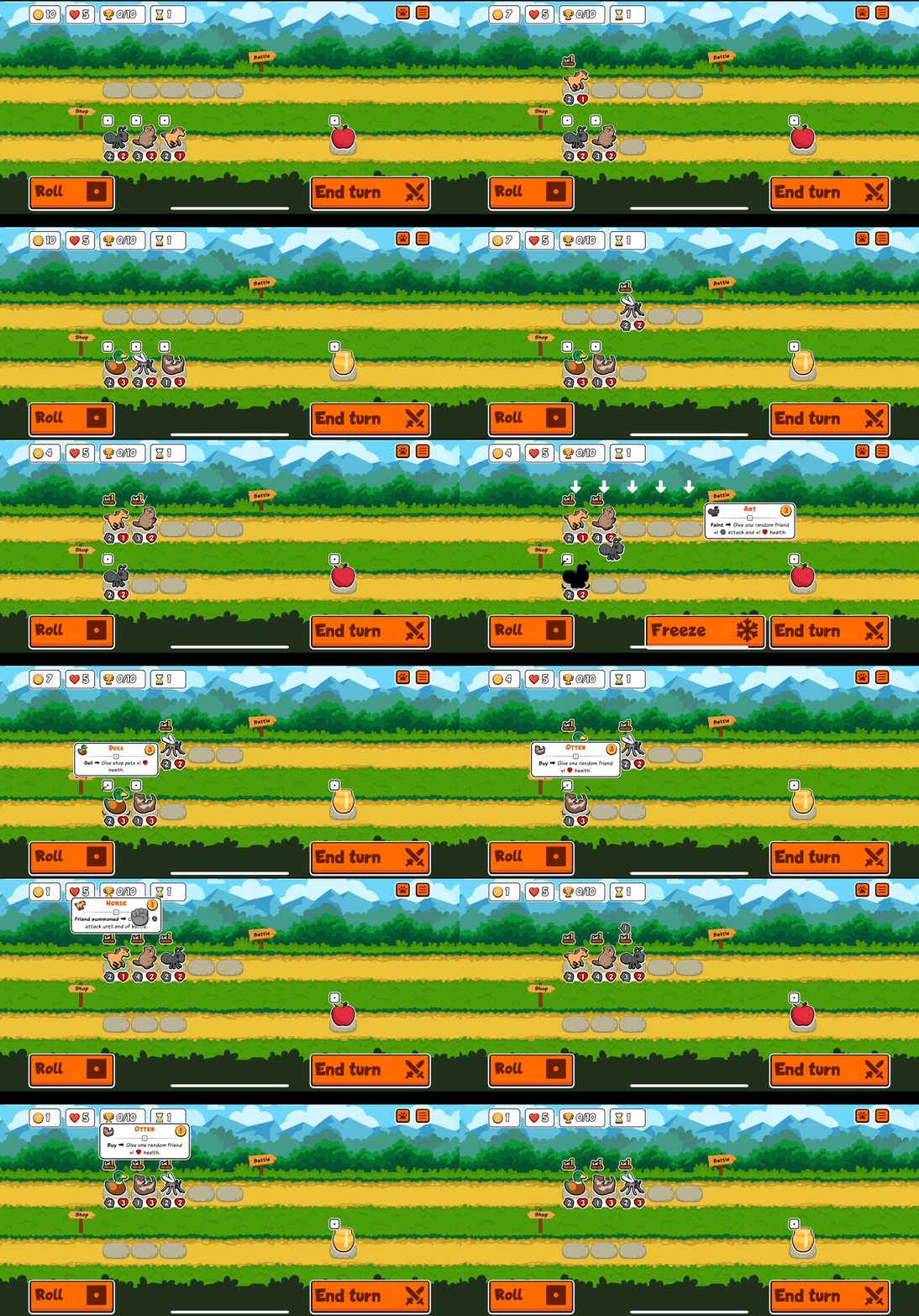
(1) you add pets to your team. You choose what order to add pets in, and what order the pets are placed in your team. Pets have certain effects that are triggered when they are added to a team.
Here’s an example of two team constructions. As you can see, the horse has triggers when pets are added after it, and the otter has a trigger when it is added to the team.

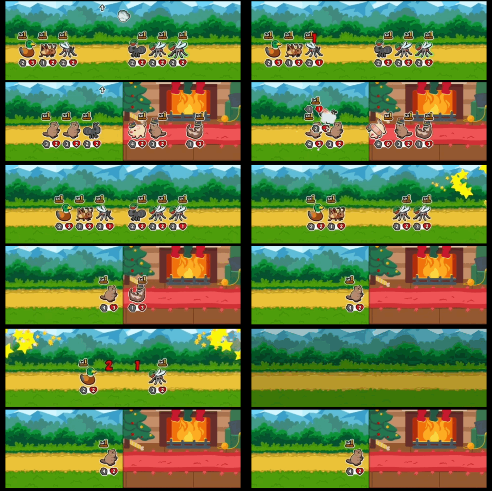
(2) Your team battles another team. The other team you are battling isn’t known to you at the time of the battle (we can pretend that you and the opponent simultaneously pick your teams as per (1) then battle). Some pets (like the Mosquito) have start-of-round effects that trigger before the actual battling begins.
During the battle the front pets of each team simultaneously deal damage to each other. The damage dealt is equal to the pets attack stat and decreases the health of the pet receiving the damage. Once a pet is out of health it faints. Throughout the battle pets might have special abilities that get triggered (like the Ant and Cricket)

A Single Round Super Auto Pets Game
Lets imagine a simplified version of this game where we only play a single round of the game and in the first stage of the game we can choose any of the possible round 1 pets that might appear. We’ll try and analyze the strategies/teams each player can pick and look for equillibria. Lets take a look at the full set of pets available in round 1.
| pet | attack | health | trigger | ability |
|---|---|---|---|---|
| 🐜 | 2 | 1 | Faint | Give one random friend +2 Attack and +1 Health |
| 🦆 | 2 | 3 | Sell | Give shop pets +1 Health |
| 🦟 | 2 | 2 | Start of battle | Deal 1 Damage to one random enemy |
| 🐎 | 2 | 1 | Friend summoned | Give it +1 Attack until end of battle |
| 🦦 | 1 | 2 | Buy | Give one random friend +1 Attack and +1 Health |
| 🦫 | 3 | 2 | Sell | Give two random friends +1 Health |
| 🦗 | 2 | 1 | Faint | Summon one 1/1 Zombie Cricket (doesn’t respawn when killed) |
| 🐟 | 2 | 2 | Level up | Give all friends +1 Attack and +1 Health |
| 🐖 | 4 | 1 | Sell | Gain +1 Gold |
Since we only care about the first round we can ignore sell triggers (🦆, 🦫) or level up triggers (🐟). Additionally the 🐖 effect isn’t as helpful as we only play one round so the +1 gold doesn’t do much in our simplified game. We’ll simulate all possible teams against each other and analyze the results.
There are 4374 teams that we will consider. There are 9 choices for each team slot (in the first round we can only afford 3 pets and buying fewer than 3 pets can’t help improve a team’s round one win probability), and there are 6 orderings of purchase (ordering of purchase matters due to the way that the buy triggers work). There are a few cases where purchasing ordering doesn’t matter but this won’t really be a big deal to double count these.
Here’s an example of a team battle:
🦆 bought 1st, 🐟 bought 2nd, 🦫 bought 3rd,
VS
🐖 bought 1st, 🦗 bought 2nd, 🐖 bought 3rd,

start 🐖(4,1) 🦗(1,2) 🐖(4,1)   VS  🦫(3,2) 🐟(2,2) 🦆(2,3)
start 	🐖(4,1) 🦗(1,2) 🐖(4,1)   VS  🦫(3,2) 🐟(2,2) 🦆(2,3)
play  		🐖(4,1) 🦗(1,2) 🐖(4,1)   VS  🦫(3,2) 🐟(2,2) 🦆(2,3)
play  			🐖(4,1) 🦗(1,2)   VS  🐟(2,2) 🦆(2,3)
play  				🐖(4,1) 🦗(1,1)   VS  🐟(2,1) 🦆(2,3)
play  					🐖(4,1)   VS  🦆(2,3)
play  						  VS
						 0.5
0.5
The above output shows the game tree where indented lines indicate game subtrees.
Here there is only one path because the entire battle is deterministic but to solve for the exact probability of a team’s win when the team has some random effects, we have to compute the possible branches and the win probabilites along each of the branches. Although we could estimate the probabilities by repeated simulation, the error on these estimates might be high enough for us to have a hard time eliminating weakly dominated strategies.
Here’s a log including pets with nondeterministic triggers (🐜 and 🦟)
🦆 bought 1st, 🦫 bought 2nd, 🐜 bought 3rd,
VS
🐖 bought 1st, 🐖 bought 2nd, 🦟 bought 3rd,

start 🐖(4,1) 🐖(4,1) 🦟(2,2)   VS  🐜(2,1) 🦫(3,2) 🦆(2,3)
start 	🐖(4,1) 🐖(4,1) 🦟(2,2)   VS  🐜(2,1) 🦫(3,2) 🦆(2,2)
play  		🐖(4,1) 🐖(4,1) 🦟(2,2)   VS  🐜(2,1) 🦫(3,2) 🦆(2,2)
play  			🐖(4,1) 🐖(4,1)   VS  🦫(3,2) 🦆(4,3)
play  				🐖(4,1)   VS  🦆(4,3)
play  					  VS
					 0.5
play  			🐖(4,1) 🐖(4,1)   VS  🦫(5,3) 🦆(2,2)
play  				🐖(4,1)   VS  🦆(2,2)
play  					  VS
					 0.5
start 	🐖(4,1) 🐖(4,1) 🦟(2,2)   VS  🐜(2,1) 🦫(3,1) 🦆(2,3)
play  		🐖(4,1) 🐖(4,1) 🦟(2,2)   VS  🐜(2,1) 🦫(3,1) 🦆(2,3)
play  			🐖(4,1) 🐖(4,1)   VS  🦫(3,1) 🦆(4,4)
play  				🐖(4,1)   VS  🦆(4,4)
play  					  VS
					 0.5
play  			🐖(4,1) 🐖(4,1)   VS  🦫(5,2) 🦆(2,3)
play  				🐖(4,1)   VS  🦆(2,3)
play  					  VS
					 0.5
start 	🐖(4,1) 🐖(4,1) 🦟(2,2)   VS  🐜(2,0) 🦫(3,2) 🦆(2,3)
play  		🐖(4,1) 🐖(4,1) 🦟(2,2)   VS  🦫(3,2) 🦆(4,4)
play  			🐖(4,1) 🐖(4,1)   VS  🦆(4,4)
play  				🐖(4,1)   VS
				 1.0
play  		🐖(4,1) 🐖(4,1) 🦟(2,2)   VS  🦫(5,3) 🦆(2,3)
play  			🐖(4,1) 🐖(4,1)   VS  🦫(5,1) 🦆(2,3)
play  				🐖(4,1)   VS  🦆(2,3)
play  					  VS
					 0.5
0.5833333333333334
The above log reflects three possibilities for which pet the Mosquito deals damage to, and then a second branch reflecting which teammate the ant gives health to. It looks like in the case where the mosquito hits the ant, then team 1 wins, but otherwise it ends in a draw.
There are also non-deterministic buy triggers.
Imagine we have
🦗 bought 1st, 🦫 bought 3rd, 🦦 bought 2nd,
VS
🐖 bought 1st, 🦆 bought 2nd, 🦦 bought 3rd,

start 🦗(2,3) 🦫(3,2) 🦦(1,2)   VS  🦦(1,2) 🦆(2,3) 🐖(5,2)
start 	🦗(2,3) 🦫(3,2) 🦦(1,2)   VS  🦦(1,2) 🦆(2,3) 🐖(5,2)
play  		🦗(2,3) 🦫(3,2) 🦦(1,2)   VS  🦦(1,2) 🦆(2,3) 🐖(5,2)
play  			🦗(2,3) 🦫(3,2) 🦦(1,1)   VS  🦦(1,1) 🦆(2,3) 🐖(5,2)
play  				🦗(2,3) 🦫(3,2)   VS  🦆(2,3) 🐖(5,2)
play  					🦗(2,3)   VS  🐖(5,2)
play  						🦗(1,1)   VS
						 1.0
start 🦗(2,3) 🦫(3,2) 🦦(1,2)   VS  🦦(1,2) 🦆(3,4) 🐖(4,1)
start 	🦗(2,3) 🦫(3,2) 🦦(1,2)   VS  🦦(1,2) 🦆(3,4) 🐖(4,1)
play  		🦗(2,3) 🦫(3,2) 🦦(1,2)   VS  🦦(1,2) 🦆(3,4) 🐖(4,1)
play  			🦗(2,3) 🦫(3,2) 🦦(1,1)   VS  🦦(1,1) 🦆(3,4) 🐖(4,1)
play  				🦗(2,3) 🦫(3,2)   VS  🦆(3,4) 🐖(4,1)
play  					🦗(2,3)   VS  🦆(3,1) 🐖(4,1)
play  						🦗(1,1)   VS  🐖(4,1)
play  							  VS
							 0.5
0.75
here there are only two non-deterministic branches based on whether team 2’s otter buffs the pig or duck (team 1’s otter will always buff the cricket). In the case where the team 2 otter makes the pig stronger then team 2 wins but otherwise it is a draw.
For each combination of two teams we simulate the outcome and end up with a 4374 by 4374 matrix \(P\) where \(P_{i,j} = \mathbb{P}(\) Team i beats Team j \()\)
Team Matchups
Once we have our matrix \(P\), if we consider two vectors \(\textbf{a}, \textbf{b} \in \mathbb{R}_{\geq 0}^{n}\) with \(\|\textbf{a}\| = \|\textbf{b}\| = 1\) where \(\textbf{a}_i, \textbf{b}_i\) is the probability that player a and player b respectively choose team choice \(i\). Then the probability player a wins is:
\[p_{a\_win} = \textbf{a}^TP\textbf{b}\]To make this tangible, if player a knows that player b is going to uniformly randomly pick a team, we can find the optimal team for player a to pick by right multiplying \(P\) by a uniform distribution to get some vector \(c\) and picking a distribution of teams \(a\) that has highest dot product with \(c\) (which would be 0 everywhere and 1 at the index where \(c\) has maximum entry)
Team: 🦗 bought 2nd, 🐜 bought 1st, 🦆 bought 3rd,
Win %: 91
and the worst team (for fun)
Team: 🐜 bought 2nd, 🐎 bought 3rd, 🦦 bought 1st,
Win %: 8
This makes sense as buying the horse last and otter first means their special abilities aren’t used at all.
Next, lets assume we are playing strategic players.
We can think of this as a matrix game where one player chooses a row of \(P\), and another player chooses a column simultaneously. Lets first look for pure Nash Equillibria. One necessary condition for this is that there is some strategy for player \(b\) such that \(a\) can’t do better than 0.5 (and the symmetric condition for \(a\)).
A symmetric game like this needs to have all of its equillibria at 0.5 otherwise the disadvantaged player can deviate to match the opponent and have a 0.5 win %. Player 1 can always deviate from a given strategy to get a better win rate (and symmetrically for the other player).
worst best response that a has to b's strategy gives a a win probability of 0.75
Looks like there are no pure equillibria. Next we iteratively remove strategies (rows and columns) from \(P\) which are dominated. This reduced matrix will make it easier for us to do further analysis.
new matrix size: 605
In our simplified matrix, against a uniform distribution of undominated teams we get a different optimal team
team: 🐎 bought 1st, 🦗 bought 2nd, 🦗 bought 3rd, with win prob of 0.804
and a different worst team (which makes sense as our old worst team was clearly dominated)
team: 🐖 bought 1st, 🐖 bought 2nd, 🦦 bought 3rd, with win prob of 0.155
Next with our simplified matrix we can look for a mixed equillibrium (where players randomly choose a team to play according to some distribution)
For more complicated mixed equillibria we can modify a code snippet from (https://code.activestate.com/recipes/496825-game-theory-payoff-matrix-solver/) to compute this
We get the following mixed strategy
prob: 34.9   team 🦟 bought 1st, 🦟 bought 2nd, 🦟 bought 3rd,
prob: 15.7   team 🦆 bought 2nd, 🐜 bought 1st, 🦆 bought 3rd,
prob: 15.0   team 🦦 bought 3rd, 🦦 bought 2nd, 🦆 bought 1st,
prob: 11.6   team 🦗 bought 3rd, 🐜 bought 1st, 🐜 bought 2nd,
prob: 6.5   team 🦦 bought 2nd, 🐜 bought 3rd, 🦟 bought 1st,
prob: 6.5   team 🦦 bought 2nd, 🐜 bought 3rd, 🦆 bought 1st,
prob: 4.0   team 🦦 bought 2nd, 🦆 bought 1st, 🦆 bought 3rd,
prob: 2.0   team 🦦 bought 2nd, 🦆 bought 1st, 🐜 bought 3rd,
prob: 1.6   team 🦦 bought 2nd, 🦆 bought 3rd, 🐜 bought 1st,
prob: 1.0   team 🦦 bought 2nd, 🦟 bought 3rd, 🦟 bought 1st,
prob: 0.5   team 🦆 bought 2nd, 🦆 bought 3rd, 🐜 bought 1st,
prob: 0.4   team 🦗 bought 2nd, 🐎 bought 1st, 🦆 bought 3rd,
prob: 0.3   team 🦗 bought 2nd, 🐜 bought 1st, 🦆 bought 3rd,
We can test a few strategies against this equillibrium. Lets see what the best pure strategy is against this distribution. A necessary condition is that it can’t do better than \(0.5\) win probability
best response is team: 🦟 bought 1st, 🦟 bought 2nd, 🦟 bought 3rd, with win prob of 0.5
Note that against our equillibrium, since the best pure strategy gives win probability of 0.5, it must be the case that the best mixed strategy can’t do better than 50%. This has to be true as the best mixed strategy’s win probability is an average of terms each of which is \(< 0.5\)
Just for fun, we can see that if we play 🦟🦟🦟 all the time its not too hard for someone to beat this with 🦆🦆🦆.
best response to best response is team: 🦆 bought 1st, 🦆 bought 2nd, 🦆 bought 3rd, with win prob of 0.8889
Against a uniform distribution the mixed strategy also does reasonably well (though we know we could do better against a uniform distribution).
73.56 %
How does this strategy translate to actually playing Super Auto Pets
The two main differences between our simplified game and the actual Super Auto Pets game are:
-
In our game there is a single round (so pet abilities that make your team stonger in future rounds are functionally ignored)
-
In our game players can choose any pets to form their team but in the game there is a randomly generated limited selection of pets
These are pretty big differences but there are some initial takeaways.
Looking at the simplified game the lack of pure equillibria tells us that there are no “broken” teams such that if you play them you will always at least draw.
Our baseline of how a team does against a randomly chosen team might give us an idea of how we expect to perform against an opponent that has a very limited random selection of teams (because of (2)).
The composition of the mixed strategy Nash equillibrium also gives us some interesting intuition as to what your opponent can exploit if you systematically underplay one of the options (for example it is interesting that some of the elements of the strategy contain 🦗 in the last position and 🐎 second to last).
Acknowledgements
Super Auto Pets was created by and is the property of Team Woods Games https://teamwoodgames.com/ - screenshots come from the iOS version of the game.