Do Distances in Manhattan Resemble the Manhattan Distance?

June 23rd , 2023 by Rohan Rao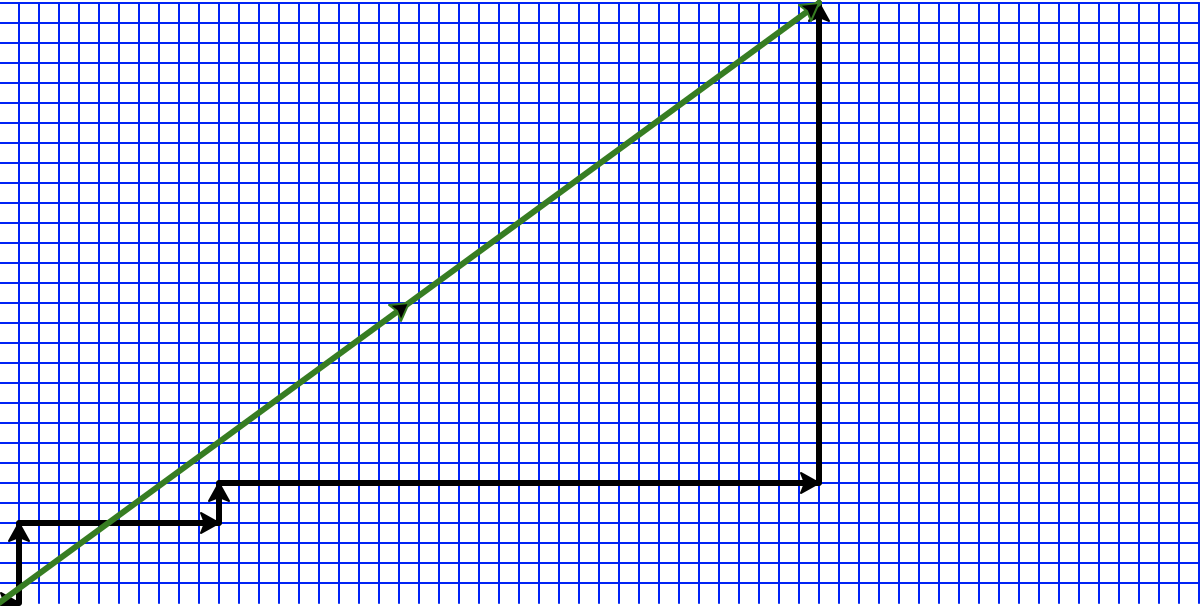

Manhattan Distance

I’m a resident of Manhattan and no stranger to the \(L_1\) distance, or ‘Manhattan’ distance. Formally the \(L_1\) distance between points in the xy plane \(a = (x_1, y_1)\) and \(b = (x_2, y_2)\) is

\[d_{L_1}(a,b) = |x_1 - x_2| + |y_1 - y_2|\]

Some of the inspiration behind calling this the manhattan distance is that if we imagine manhattan as a grid (where streets run in the \(x\) and \(y\) direction) of square 1 x 1 blocks, the \(L_1\) distance indicates the shortest path between points on the grid.

Manhattan does consist of a pretty defined grid structure of streets but not quite a perfect grid of blocks. I am interested in how well the \(L_1\) distance aligns to shortest paths on the true Manhattan Grid.

As another candidate for a distance that might capture how far away things are is the \(L_2\) distance:

\[d_{L_2}(a,b) = \sqrt{(x_1 - x_2)^2 + (y_1 - y_2)^2}\]

Which is the straightline distance between the points

In the post thumbnail the green line depicts the shortest path between a pair of points according to the \(L_2\) distance, and the black line indicates a (not unique!) shortest path according to the \(L_1\) distance.

Data

We start by loading the open street map data for Manhattan. This gives us a graph which represents the street structure of New York. Vertices of the graph have lat/long data to indicate their position on the globe and the edges represent streets between these points (and we have info about the length of the edges).

Here’s an example of the adjacency info for the graph

{'n': 4494,
 'm': 9714,
 'k_avg': 4.3230974632843795,
 'edge_length_total': 1144636.418000003,
 'edge_length_avg': 117.83368519662375,
 'streets_per_node_avg': 3.576101468624833,
 'streets_per_node_counts': {0: 0,
  1: 78,
  2: 25,
  3: 1688,
  4: 2639,
  5: 61,
  6: 3},
 'streets_per_node_proportions': {0: 0.0,
  1: 0.017356475300400534,
  2: 0.0055629728526924785,
  3: 0.3756119270137962,
  4: 0.5872274143302181,
  5: 0.013573653760569649,
  6: 0.0006675567423230974},
 'intersection_count': 4416,
 'street_length_total': 959830.5300000011,
 'street_segment_count': 7988,
 'street_length_avg': 120.1590548322485,
 'circuity_avg': 1.0184236347849767,
 'self_loop_proportion': 0.00100150225338007}

here’s the drawn graph (with vertices in their correct position) below

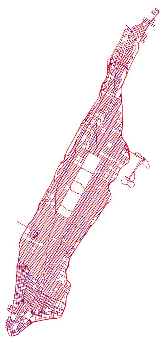
We can load these into a geo-dataframe for analysis.

For example, here’s a sample of the vertex data.

	x	y
osmid
42421728	-73.960044	40.798048
42421731	-73.961474	40.798654
42421737	-73.962873	40.799244
42421741	-73.965691	40.800429
42421745	-73.967996	40.801398

And heres some edge data

			name	oneway	length
u	v	key
42421728	42432736	0	Central Park West	False	86.258
	42435337	0	Central Park West	False	85.345
	42421731	0	West 106th Street	False	138.033
42421731	42437916	0	Manhattan Avenue	False	86.149
	42432737	0	Manhattan Avenue	False	85.611

Although many of the vertices in the graph are on intersections, some of the vertices are on curved roads. we could condense some of these vertices but that might risk distorting some of the distances so I’m opting to keep the graph as is. The main preprocessing we do is making sure our directed graph is strongly connected.

True Manhattan Distances between vertices

To start with I’ll compute pairwise shortest distances between vertices in the graph. This will serve as the ground truth for how the \(L_1\) distance measures up. We’ll use repeated Dijkstra’s algorithm for this since the graph is sparse.

We’ll also find shortest paths on an undirected version of the graph. Since our graph is intended to show driveable streets and paths it takes into account one-way roads. Just from the perspective of a pedestrian and assuming we have sidewalks everywhere it’s not unreasonable to consider the graph undirected. (I think osmnx has a walking version of the graph but we are just going to make all the edges in the driving graph undirected).

As a sanity check we can compare the shortest path distances (which are in meters) to the google maps distance for a few points. (we’ll use the undirected graph distances for these so we can use the google maps walking distance)

[[ 40.7976795 -73.9372797]
 [ 40.7472997 -73.9740676]]
6401.876 meters

On Google Maps this is 6437.38 meters walking

[[ 40.7980478 -73.9600437]
 [ 40.7850352 -73.9806732]]
2894.3380000000006 meters

Google Maps calls this 2896.82 meters.

[[ 40.7196963 -74.0059515]
 [ 40.8253247 -73.9457322]]
13240.130000000008 meters

This is 13196.6 meters walking on Google Maps

These seem to be pretty close so this is probably a fine ground truth to compare our other metrics against

\(L_1\) distances between vertices

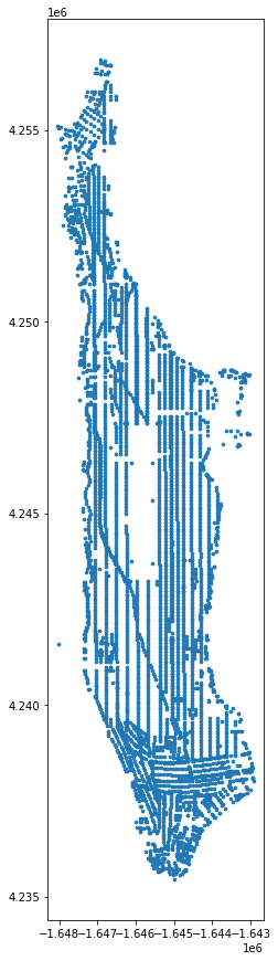
First we will compute the \(L_1\) distance between the vertices in the graph. Our vertices have locations specified as latitudes and longitudes so first we want to map these locations into the xy plane using a standard map projection

Then we will rotate Manhattan 28.6ish degrees such that most of the city blocks look aligned to the axes of the Cartesian grid. Next we will compute the pairwise \(L_1\) distances. It’s worth noting that the rotation we choose matters since rotating the points doesn’t preserve the \(L_1\) distances between them.

\(L_2\) distance

For good measure lets also compute \(L_2\) distances as a baseline

Comparing the Distances

For each candidate distance \(d\) between pair of points \(a,b\) we will compute the similarity as

\[\Delta_d(a,b) = \frac{d(a,b)}{s(a,b)}\]

wherer \(s\) is the graph shortest path (either directed or undirected). \(\Delta\) near 1 is better. We pick this because we want a metric somewhat invariant to the scale of the distances. This definition also has some inspiration from the way that distortion between metric spaces is defined. Additionally we can interpret this in percentage terms ((\(1-\Delta\)) is the percent error)

Directed

Avg delta L_1: 1.0064148760344036 inflated by 0.64%  stdev of 0.10262369325206665
Avg delta L_2: 0.8495350380443217 deflated by -15.04%  stdev of 0.10770066103181529

Overall the \(L_1\) distance does line up to empirical manhattan distances better than the \(L_2\) distance

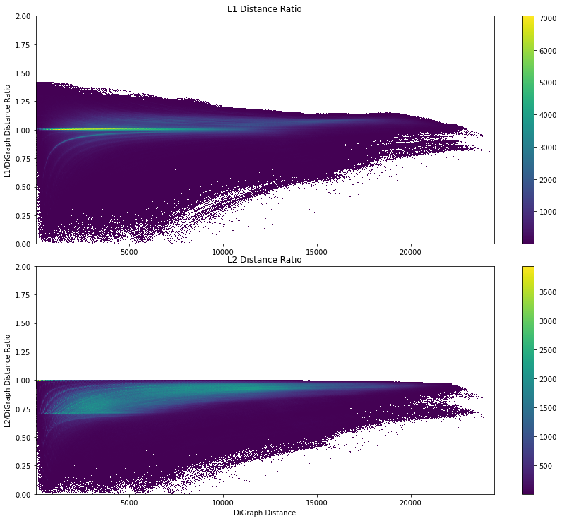
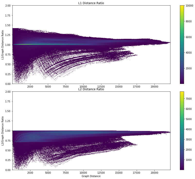
When plotting our ratios as a function of graph distance this also confirms this.

It does look for both graphs like there is less variance as the graph distance gets longer (maybe because the distribution of points that are very far away from each other looks special, or this might be explained by longer distances smoothing out some errors).

Near 0 we see more variance in the ratios (maybe because small noise or error components end up being larger percentages of the graph distances).

There also seem to be certain visual effects (looks like there are certain sets of points in the plot that form patterns or lines) that I’d think are probably a result of certain points corresponding to subpaths of shortest paths represented by other points in the plot.

We can look at some summary statistics at different “true manhattan” distance ranges.

> 17000
L1 mean: 1.056 L2 mean: 0.934
L1 std: 0.047 L2 std: 0.044

10,000 - 17,000
L1 mean: 1.027 L2 mean: 0.909
L1 std: 0.072 L2 std: 0.07

1,000 - 10,000
L1 mean: 1.0 L2 mean: 0.83
L1 std: 0.105 L2 std: 0.106

100 - 1,000
L1 mean: 0.919 L2 mean: 0.743
L1 std: 0.203 L2 std: 0.173

<100
L1 mean: 1.077 L2 mean: 0.966
L1 std: 0.149 L2 std: 0.093

Interestingly at a glance it also seems like the \(L_2\) distance seems to do better at very long graph distances or very short ones (in the latter case even doing better than the \(L_1\) distance).

The latter fact isn’t that surprising because the smallest paths on the graph will contain a single edge whose length will be roughly the \(L_2\) distance.

Undirected

Avg undirected delta L_1: 1.0489620755405908 inflated by 4.89%  stdev of 0.07860555603160621
Avg undirected delta L_2: 0.8846728750571392 deflated by -11.53%  stdev of 0.08723663701126477

These graphs have similarities to the previous pair but since these are undirected distances we see a narrower range of distance ratios. In the undirected case the \(L_2\) distance does better than it did in the directed case. I don’t think this is that unexpected. The more effective roads we add in between points, the better the \(L_2\) distance should look generally.

At really far distances the \(L_2\) distance even looks better than the \(L_1\) distance.

> 17000
L1 mean: 1.079 L2 mean: 0.956
L1 std: 0.028 L2 std: 0.02

10,000 - 17,000
L1 mean: 1.054 L2 mean: 0.934
L1 std: 0.061 L2 std: 0.056

1,000 - 10,000
L1 mean: 1.048 L2 mean: 0.869
L1 std: 0.081 L2 std: 0.087

100 - 1,000
L1 mean: 1.019 L2 mean: 0.826
L1 std: 0.125 L2 std: 0.119

<100
L1 mean: 1.085 L2 mean: 0.971
L1 std: 0.134 L2 std: 0.072

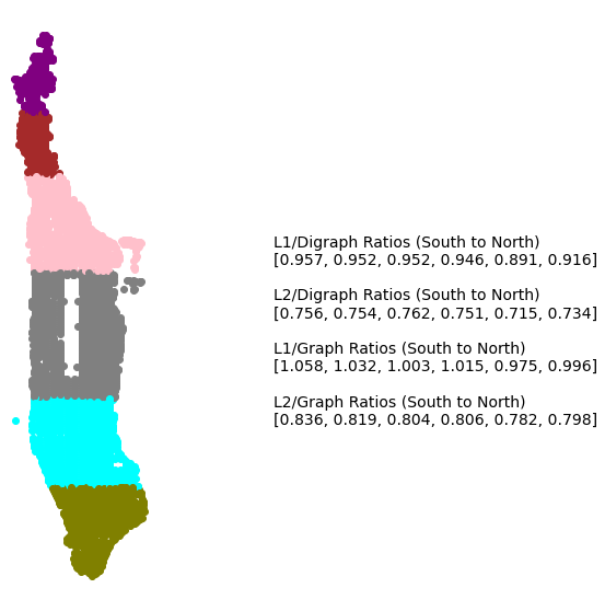
Regions of Manhattan

Another way we can analyze the errors is by the region of Manhattan that we are looking at. If a path exists in the middle of manhattan where the grid structure of streets is prominant, then maybe the \(L_2\) distance is much better in these regions. At the tips of Manhattan the grid structure might break down and the \(L_2\) distance might be better if there are a lot more streets going directly from point \(a\) to \(b\).

To do this we can bucket the \(y\) axis into a few bins and then look at the errors for paths in these regions (one side effect of this is that we won’t consider the paths crossing between these sections).

Is it reasonable to say the Manhattan distance is the \(L_1\) distance

I think so! It seems like for the most part the \(L_1\) distance outperforms one of the few distance metrics more popular than it (\(L_2\)) but there are a few places where the \(L_2\) distance might be reasonable instead. One limitation of this discussion is that our selection of reference points to compute distances between could have some bias and I didn’t really try other methods of generating this set. I won’t go too much into it but as a thought experiment, if we added a lot of points along a long diagonal road, this might make the \(L_2\) distanace look better. That’s not to say that this doesn’t conclude anything but it’s certainly worth thinking about when interpreting the results and maybe fun to play around with later. Visually it looks like the intersection points of roads provide good coverage so I’ll say at a first glance the \(L_1\) distance tentatively looks better even given this qualification.

Data Sources and Acknowledgements

All the data used here comes from Open Street Map API https://osmnx.readthedocs.io/en/stable/